Java HashMap底层实现原理

本节用于记录Java HashMap底层数据结构、方法实现原理等，基于JDK 1.8。

底层数据结构

Java HashMap底层采用哈希表结构（数组+链表、JDK1.8后为数组+链表或红黑树）实现，结合了数组和链表的优点：

1. 数组优点：通过数组下标可以快速实现对数组元素的访问，效率极高；

2. 链表优点：插入或删除数据不需要移动元素，只需修改节点引用，效率极高。

HashMap图示如下所示：

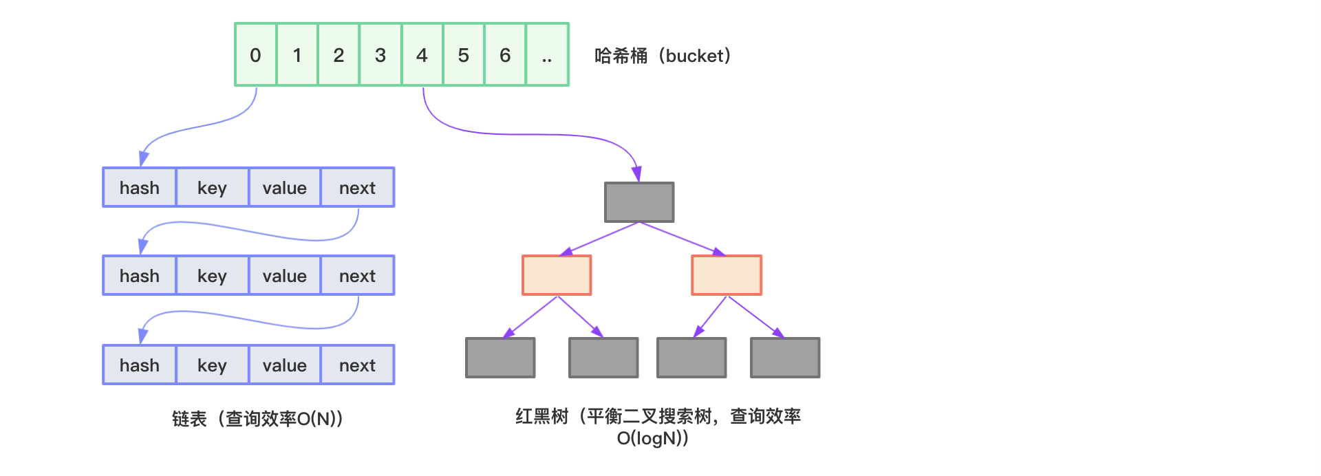
HashMap内部使用数组存储数据，数组中的每个元素类型为Node<K,V>：

static class Node<K,V> implements Map.Entry<K,V> {
    final int hash;
    final K key;
    V value;
    Node<K,V> next;

    Node(int hash, K key, V value, Node<K,V> next) {
        this.hash = hash;
        this.key = key;
        this.value = value;
        this.next = next;
    }

    public final K getKey()        { return key; }
    public final V getValue()      { return value; }
    public final String toString() { return key + "=" + value; }

    public final int hashCode() {
        return Objects.hashCode(key) ^ Objects.hashCode(value);
    }

    public final V setValue(V newValue) {
        V oldValue = value;
        value = newValue;
        return oldValue;
    }

    public final boolean equals(Object o) {
        if (o == this)
            return true;
        if (o instanceof Map.Entry) {
            Map.Entry<?,?> e = (Map.Entry<?,?>)o;
            if (Objects.equals(key, e.getKey()) &&
                Objects.equals(value, e.getValue()))
                return true;
        }
        return false;
    }
}

Node包含了四个字段：hash、key、value、next，其中next表示链表的下一个节点。

HashMap通过hash方法计算key的哈希码，然后通过(n-1)&hash公式（n为数组长度）得到key在数组中存放的下标。当两个key在数组中存放的下标一致时，数据将以链表的方式存储（哈希冲突，哈希碰撞）。我们知道，在链表中查找数据必须从第一个元素开始一层一层往下找，直到找到为止，时间复杂度为O(N)，所以当链表长度越来越长时，HashMap的效率越来越低。

为了解决这个问题，JDK1.8开始采用数组+链表+红黑树的结构来实现HashMap。当链表中的元素超过8个（TREEIFY_THRESHOLD）并且数组长度大于64（MIN_TREEIFY_CAPACITY）时，会将链表转换为红黑树，转换后数据查询时间复杂度为O(logN)。

红黑树的节点使用TreeNode表示：

static final class TreeNode<K,V> extends LinkedHashMap.Entry<K,V> {
    TreeNode<K,V> parent;  // red-black tree links
    TreeNode<K,V> left;
    TreeNode<K,V> right;
    TreeNode<K,V> prev;    // needed to unlink next upon deletion
    boolean red;
    TreeNode(int hash, K key, V val, Node<K,V> next) {
        super(hash, key, val, next);
    }
    ...
}

HashMap包含几个重要的变量：

// 数组默认的初始化长度16
static final int DEFAULT_INITIAL_CAPACITY = 1 << 4;

// 数组最大容量，2的30次幂，即1073741824
static final int MAXIMUM_CAPACITY = 1 << 30;

// 默认加载因子值
static final float DEFAULT_LOAD_FACTOR = 0.75f;

// 链表转换为红黑树的长度阈值
static final int TREEIFY_THRESHOLD = 8;

// 红黑树转换为链表的长度阈值
static final int UNTREEIFY_THRESHOLD = 6;

// 链表转换为红黑树时，数组容量必须大于等于64
static final int MIN_TREEIFY_CAPACITY = 64;

// HashMap里键值对个数
transient int size;

// 扩容阈值，计算方法为 数组容量*加载因子
int threshold;

// HashMap使用数组存放数据，数组元素类型为Node<K,V>
transient Node<K,V>[] table;

// 加载因子
final float loadFactor;

// 用于快速失败，由于HashMap非线程安全，在对HashMap进行迭代时，如果期间其他线程的参与导致HashMap的结构发生变化了（比如put，remove等操作），直接抛出ConcurrentModificationException异常
transient int modCount;

上面这些字段在下面源码解析的时候尤为重要，其中需要着重讨论的是加载因子是什么，为什么默认值为0.75f。

加载因子也叫扩容因子，用于决定HashMap数组何时进行扩容。比如数组容量为16，加载因子为0.75，那么扩容阈值为16*0.75=12，即HashMap数据量大于等于12时，数组就会进行扩容。我们都知道，数组容量的大小在创建的时候就确定了，所谓的扩容指的是重新创建一个指定容量的数组，然后将旧值复制到新的数组里。扩容这个过程非常耗时，会影响程序性能。所以加载因子是基于容量和性能之间平衡的结果：

• 当加载因子过大时，扩容阈值也变大，也就是说扩容的门槛提高了，这样容量的占用就会降低。但这时哈希碰撞的几率就会增加，效率下降；
• 当加载因子过小时，扩容阈值变小，扩容门槛降低，容量占用变大。这时候哈希碰撞的几率下降，效率提高。

可以看到容量占用和性能是此消彼长的关系，它们的平衡点由加载因子决定，0.75是一个即兼顾容量又兼顾性能的经验值。

此外用于存储数据的table字段使用transient修饰，通过transient修饰的字段在序列化的时候将被排除在外，那么HashMap在序列化后进行反序列化时，是如何恢复数据的呢？HashMap通过自定义的readObject/writeObject方法自定义序列化和反序列化操作。这样做主要是出于以下两点考虑：

1. table一般不会存满，即容量大于实际键值对个数，序列化table未使用的部分不仅浪费时间也浪费空间；
2. key对应的类型如果没有重写hashCode方法，那么它将调用Object的hashCode方法，该方法为native方法，在不同JVM下实现可能不同；换句话说，同一个键值对在不同的JVM环境下，在table中存储的位置可能不同，那么在反序列化table操作时可能会出错。

所以在HashXXX类中（如HashTable，HashSet，LinkedHashMap等等），我们可以看到，这些类用于存储数据的字段都用transient修饰，并且都自定义了readObject/writeObject方法。readObject/writeObject方法这节就不进行源码分析了，有兴趣自己研究。

put源码

put方法源码如下：

public V put(K key, V value) {
    return putVal(hash(key), key, value, false, true);
}

put方法通过hash函数计算key对应的哈希值，hash函数源码如下：

static final int hash(Object key) {
    int h;
    return (key == null) ? 0 : (h = key.hashCode()) ^ (h >>> 16);
}

如果key为null，返回0，不为null，则通过(h = key.hashCode()) ^ (h >>> 16)公式计算得到哈希值。该公式通过hashCode的高16位异或低16位得到哈希值，主要从性能、哈希碰撞角度考虑，减少系统开销，不会造成因为高位没有参与下标计算从而引起的碰撞。

得到key对应的哈希值后，再调用putVal(hash(key), key, value, false, true)方法插入元素：

final V putVal(int hash, K key, V value, boolean onlyIfAbsent,
               boolean evict) {
    Node<K,V>[] tab; Node<K,V> p; int n, i;
    // 如果数组(哈希表)为null或者长度为0，则进行数组初始化操作
    if ((tab = table) == null || (n = tab.length) == 0)
        n = (tab = resize()).length;
    // 根据key的哈希值计算出数据插入数组的下标位置，公式为(n-1)&hash
    if ((p = tab[i = (n - 1) & hash]) == null)
        // 如果该下标位置还没有元素，则直接创建Node对象，并插入
        tab[i] = newNode(hash, key, value, null);
    else {
        Node<K,V> e; K k;
        // 如果目标位置key已经存在，则直接覆盖
        if (p.hash == hash &&
            ((k = p.key) == key || (key != null && key.equals(k))))
            e = p;
        // 如果目标位置key不存在，并且节点为红黑树，则插入红黑树中
        else if (p instanceof TreeNode)
            e = ((TreeNode<K,V>)p).putTreeVal(this, tab, hash, key, value);
        else {
            // 否则为链表结构，遍历链表，尾部插入
            for (int binCount = 0; ; ++binCount) {
                if ((e = p.next) == null) {
                    p.next = newNode(hash, key, value, null);
                    // 如果链表长度大于等于TREEIFY_THRESHOLD，则考虑转换为红黑树
                    if (binCount >= TREEIFY_THRESHOLD - 1) // -1 for 1st
                        treeifyBin(tab, hash); // 转换为红黑树操作，内部还会判断数组长度是否小于MIN_TREEIFY_CAPACITY，如果是的话不转换
                    break;
                }
                // 如果链表中已经存在该key的话，直接覆盖替换
                if (e.hash == hash &&
                    ((k = e.key) == key || (key != null && key.equals(k))))
                    break;
                p = e;
            }
        }
        if (e != null) { // existing mapping for key
            // 返回被替换的值
            V oldValue = e.value;
            if (!onlyIfAbsent || oldValue == null)
                e.value = value;
            afterNodeAccess(e);
            return oldValue;
        }
    }
    // 模数递增
    ++modCount;
    // 当键值对个数大于等于扩容阈值的时候，进行扩容操作
    if (++size > threshold)
        resize();
    afterNodeInsertion(evict);
    return null;
}

put操作过程总结：

1. 判断HashMap数组是否为空，是的话初始化数组（由此可见，在创建HashMap对象的时候并不会直接初始化数组）；
2. 通过(n-1) & hash计算key在数组中的存放索引；
3. 目标索引位置为空的话，直接创建Node存储；

4. 目标索引位置不为空的话，分下面三种情况：

   4.1. key相同，覆盖旧值；

   4.2. 该节点类型是红黑树的话，执行红黑树插入操作；

   4.3. 该节点类型是链表的话，遍历到最后一个元素尾插入，如果期间有遇到key相同的，则直接覆盖。如果链表长度大于等于TREEIFY_THRESHOLD，并且数组容量大于等于MIN_TREEIFY_CAPACITY，则将链表转换为红黑树结构；

5. 判断HashMap元素个数是否大于等于threshold，是的话，进行扩容操作。

get源码

get和put相比，就简单多了，下面是get操作源码：

public V get(Object key) {
    Node<K,V> e;
    return (e = getNode(hash(key), key)) == null ? null : e.value;
}

final Node<K,V> getNode(int hash, Object key) {
    Node<K,V>[] tab; Node<K,V> first, e; int n; K k;
    // 判断数组是否为空，数组长度是否大于0，目标索引位置下元素是否为空，是的话直接返回null
    if ((tab = table) != null && (n = tab.length) > 0 &&
        (first = tab[(n - 1) & hash]) != null) {
        // 如果目标索引位置元素就是要找的元素，则直接返回
        if (first.hash == hash && // always check first node
            ((k = first.key) == key || (key != null && key.equals(k))))
            return first;
        // 如果目标索引位置元素的下一个节点不为空
        if ((e = first.next) != null) {
            // 如果类型是红黑树，则从红黑树中查找
            if (first instanceof TreeNode)
                return ((TreeNode<K,V>)first).getTreeNode(hash, key);
            do {
            // 否则就是链表，遍历链表查找目标元素
                if (e.hash == hash &&
                    ((k = e.key) == key || (key != null && key.equals(k))))
                    return e;
            } while ((e = e.next) != null);
        }
    }
    return null;
}

resize源码

由前面的put源码分析我们知道，数组的初始化和扩容都是通过调用resize方法完成的，所以现在来关注下resize方法的源码：

final Node<K,V>[] resize() {
    // 扩容前的数组
    Node<K,V>[] oldTab = table;
    // 扩容前的数组的大小和阈值
    int oldCap = (oldTab == null) ? 0 : oldTab.length;
    int oldThr = threshold;
    // 预定义新数组的大小和阈值
    int newCap, newThr = 0;
    if (oldCap > 0) {
        // 超过最大值就不再扩容了
        if (oldCap >= MAXIMUM_CAPACITY) {
            threshold = Integer.MAX_VALUE;
            return oldTab;
        }
        // 扩大容量为当前容量的两倍，但不能超过 MAXIMUM_CAPACITY
        else if ((newCap = oldCap << 1) < MAXIMUM_CAPACITY &&
                 oldCap >= DEFAULT_INITIAL_CAPACITY)
            newThr = oldThr << 1; // double threshold
    }
    // 当前数组没有数据，使用初始化的值
    else if (oldThr > 0) // initial capacity was placed in threshold
        newCap = oldThr;
    else {               // zero initial threshold signifies using defaults
        // 如果初始化的值为 0，则使用默认的初始化容量，默认值为16
        newCap = DEFAULT_INITIAL_CAPACITY;
        newThr = (int)(DEFAULT_LOAD_FACTOR * DEFAULT_INITIAL_CAPACITY);
    }
    // 如果新的容量等于 0
    if (newThr == 0) {
        float ft = (float)newCap * loadFactor;
        newThr = (newCap < MAXIMUM_CAPACITY && ft < (float)MAXIMUM_CAPACITY ?
                  (int)ft : Integer.MAX_VALUE);
    }
    threshold = newThr; 
    @SuppressWarnings({"rawtypes","unchecked"})
    Node<K,V>[] newTab = (Node<K,V>[])new Node[newCap];
    // 开始扩容，将新的容量赋值给 table
    table = newTab;
    // 原数据不为空，将原数据复制到新 table 中
    if (oldTab != null) {
        // 根据容量循环数组，复制非空元素到新 table
        for (int j = 0; j < oldCap; ++j) {
            Node<K,V> e;
            if ((e = oldTab[j]) != null) {
                oldTab[j] = null;
                // 如果链表只有一个，则进行直接赋值
                if (e.next == null)
                    newTab[e.hash & (newCap - 1)] = e;
                else if (e instanceof TreeNode)
                    // 红黑树相关的操作
                    ((TreeNode<K,V>)e).split(this, newTab, j, oldCap);
                else { // preserve order
                    // 链表复制，JDK 1.8 扩容优化部分
                    Node<K,V> loHead = null, loTail = null;
                    Node<K,V> hiHead = null, hiTail = null;
                    Node<K,V> next;
                    do {
                        next = e.next;
                        // 原索引
                        if ((e.hash & oldCap) == 0) {
                            if (loTail == null)
                                loHead = e;
                            else
                                loTail.next = e;
                            loTail = e;
                        }
                        // 原索引 + oldCap
                        else {
                            if (hiTail == null)
                                hiHead = e;
                            else
                                hiTail.next = e;
                            hiTail = e;
                        }
                    } while ((e = next) != null);
                    // 将原索引放到哈希桶中
                    if (loTail != null) {
                        loTail.next = null;
                        newTab[j] = loHead;
                    }
                    // 将原索引 + oldCap 放到哈希桶中
                    if (hiTail != null) {
                        hiTail.next = null;
                        newTab[j + oldCap] = hiHead;
                    }
                }
            }
        }
    }
    return newTab;
}

JDK1.8在扩容时通过高位运算e.hash & oldCap结果是否为0来确定元素是否需要移动，主要有如下两种情况：

情况一：

扩容前oldCap=16，hash=5，(n-1)&hash=15&5=5，hash&oldCap=5&16=0；

扩容后newCap=32，hash=5，(n-1)&hash=31&5=5，hash&oldCap=5&16=0。

这种情况下，扩容后元素索引位置不变，并且hash&oldCap==0。

情况二：

扩容前oldCap=16，hash=18，(n-1)&hash=15&18=2，hash&oldCap=18&16=16；

扩容后newCap=32，hash=18，(n-1)&hash=31&18=18，hash&oldCap=18&16=16。

这种情况下，扩容后元素索引位置为18，即旧索引2加16(oldCap)，并且hash&oldCap!=0。

遍历原理

我们通常使用下面两种方式遍历HashMap：

HashMap<String, Object> map = new HashMap<>();
map.put("1", "a");
map.put("4", "d");
map.put("2", "b");
map.put("9", "i");
map.put("3", "c");

Set<Map.Entry<String, Object>> entries = map.entrySet();
for (Map.Entry<String, Object> entry : entries) {
    System.out.println(entry.getKey() + ": " + entry.getValue());
}

System.out.println("-------");

Set<String> keySet = map.keySet();
for (String key : keySet) {
    System.out.println(key + ": " + map.get(key));
}

程序输出：

1: a
2: b
3: c
4: d
9: i
-------
1: a
2: b
3: c
4: d
9: i

通过前面对put源码的分析，我们知道HashMap是无序的，输出元素顺序和插入元素顺序一般都不一样。但是多次运行上面的程序你会发现，每次遍历的顺序都是一样的。那么遍历的原理是什么，内部是如何操作的？

通过entrySet或者keySet遍历，它们的内部原理是一样的，这里以entrySet为例。

通过查看代码对应的class文件，你会发现下面这段代码实际会被转换为iterator遍历：

Set<Map.Entry<String, Object>> entries = map.entrySet();
for (Map.Entry<String, Object> entry : entries) {
    System.out.println(entry.getKey() + ": " + entry.getValue());
}

增强for循环会被编译为：

Set<Entry<String, Object>> entries = map.entrySet();
Iterator var3 = entries.iterator();

while(var3.hasNext()) {
    Entry<String, Object> entry = (Entry)var3.next();
    System.out.println((String)entry.getKey() + ": " + entry.getValue());
}

我们查看entrySet，iterator，hasNext，next方法的源码就可以清楚的了解到HashMap遍历原理了：

public Set<Map.Entry<K,V>> entrySet() {
    Set<Map.Entry<K,V>> es;
    // entrySet一开始为null，通过new EntrySet()创建
    return (es = entrySet) == null ? (entrySet = new EntrySet()) : es;
}

final class EntrySet extends AbstractSet<Map.Entry<K,V>> {
    public final int size()                 { return size; }
    public final void clear()               { HashMap.this.clear(); }
    // EntrySet内部包含迭代器方法，方法内部通过new EntryIterator()创建Entry迭代器
    public final Iterator<Map.Entry<K,V>> iterator() {
        return new EntryIterator();
    }
    ...... 
}

// EntryIterator继承自HashIterator，调用EntryIterator的hasNext方法实际调用的是
// 父类HashIterator的hashNext方法，调用EntryIterator的next方法，方法内部调用的是父类HashIterator
// 的nextNode方法，所以我们主要关注HashIterator的源码
final class EntryIterator extends HashIterator implements Iterator<Map.Entry<K,V>> {
    public final Map.Entry<K,V> next() { return nextNode(); }
}

abstract class HashIterator {
    Node<K,V> next;        // 下一个节点
    Node<K,V> current;     // 当前节点
    int expectedModCount;  // 期待的模数值，用于快速失败
    int index;             // 当前遍历的table index

    HashIterator() {
        // 将当前模数值赋值给期待的模数值，所以在遍历的时候，别的线程调用了当前hashMap实例的
        // 增删改方法，模数值会改变，那么expectedModCount和modCount就不相等了，遍历操作直接
        // 抛出ConcurrentModificationException
        expectedModCount = modCount;
        Node<K,V>[] t = table;
        current = next = null;
        // 从hashMap数组头部开始遍历
        index = 0;
        if (t != null && size > 0) { // advance to first entry
            // 从数组头部开始找，index递增，当index位置的节点不为空时，将其赋值给next
            // 也就是说，在创建hashMap迭代器的时候，内部就已经找到了hashMap数组中第一个非空节点了
            do {} while (index < t.length && (next = t[index++]) == null);
        }
    }

    public final boolean hasNext() {
        // 逻辑很简单，就是判断next是否为空
        return next != null;
    }

    final Node<K,V> nextNode() {
        Node<K,V>[] t;
        Node<K,V> e = next;
        if (modCount != expectedModCount)
            // 模数判断
            throw new ConcurrentModificationException();
        if (e == null)
            // 如果next为空了，还调用nextNode方法的话，将抛出NoSuchElementException异常
            throw new NoSuchElementException();
        // 这段逻辑也很简单，主要包含如下两种情况：
        // 1. 如果当前节点的next节点为空的话，说明该节点无需进行链表遍历了（就一个节点或者已经到了链表的末尾），那么进行do while循环，直到找到hashMap数组中下一个不为空的节点
        // 2. 如果当前节点的next节点不为空的话，说明该位置存在链表，那么外界在循环调用iterator的next方法时，实际就是不断调用nextNode方法遍历链表操作
        if ((next = (current = e).next) == null && (t = table) != null) {
            do {} while (index < t.length && (next = t[index++]) == null);
        }
        return e;
    }

    ......
}

总之，遍历HashMap的过程就是从头查找HashMap数组中的不为空的结点，如果该结点下存在链表，则遍历该链表，遍历完链表后再找HashMap数组中下一个不为空的结点，以此进行下去直到遍历结束。

那么，如果某个结点下是红黑树结构的话，怎么遍历？其实当链表转换为红黑树时，链表节点里包含的next字段信息是保留的，所以我们依旧可以通过红黑树节点中的next字段找到下一个节点。

与JDK1.7主要区别

JDK1.7 HashMap源码：https://github.com/ZhaoX/jdk-1.7-annotated/blob/master/src/java/util/HashMap.java。

数组元素类型不同

JDK1.8 HashMap数组元素类型为Node<K,V>，JDK1.7 HashMap数组元素类型为Entry<K,V>：

transient Entry<K,V>[] table = (Entry<K,V>[]) EMPTY_TABLE;

static class Entry<K,V> implements Map.Entry<K,V> {
    final K key;
    V value;
    Entry<K,V> next;
    int hash;

    ......
}

实际就是换了个类名，并没有什么本质不同。

hash计算规则不同

JDK1.7 hash计算规则为：

final int hash(Object k) {
    int h = hashSeed;
    if (0 != h && k instanceof String) {
        return sun.misc.Hashing.stringHash32((String) k);
    }

    h ^= k.hashCode();

    // This function ensures that hashCodes that differ only by
    // constant multiples at each bit position have a bounded
    // number of collisions (approximately 8 at default load factor).
    h ^= (h >>> 20) ^ (h >>> 12);
    return h ^ (h >>> 7) ^ (h >>> 4);
}

相比于JDK1.8的hash方法，JDK1.7的hash方法的性能会稍差一点。

put操作不同

JDK1.7并没有使用红黑树，如果哈希冲突后，都用链表解决。区别于JDK1.8的尾部插入，JDK1.7采用头部插入的方式：

public V put(K key, V value) {   
    // 键为null，将元素放置到table数组的0下标处
    if (key == null)  
        return putForNullKey(value); 
    // 计算hash和数组下标索引位置
    int hash = hash(key.hashCode());  
    int i = indexFor(hash, table.length);  
    // 遍历链表，当key一致时，说明该key已经存在，使用新值替换旧值并返回
    for (Entry<K,V> e = table[i]; e != null; e = e.next) {  
        Object k;  
        if (e.hash == hash && ((k = e.key) == key || key.equals(k))) {  
            V oldValue = e.value;  
            e.value = value;  
            e.recordAccess(this);  
            return oldValue;  
        }  
    }  
    
    modCount++;
    // 插入链表
    addEntry(hash, key, value, i);  
    return null;  
} 

private V putForNullKey(V value) { 
    // 一样的，新旧值替换
    for (Entry<K,V> e = table[0]; e != null; e = e.next) {  
        if (e.key == null) {  
            V oldValue = e.value;  
            e.value = value;  
            e.recordAccess(this);  
            return oldValue;  
        }  
    }  
    
    modCount++;  
    // 插入到数组下标为0位置
    addEntry(0, null, value, 0);  
    return null;  
} 

void addEntry(int hash, K key, V value, int bucketIndex) {
    // 新值头部插入，原先头部变成新的头部元素的next
    Entry<K, V> e = table[bucketIndex];
    table[bucketIndex] = new Entry<K, V>(hash, key, value, e);
    // 计数，扩容
    if (size++ >= threshold)
        resize(2 * table.length);
}

扩容操作不同

JDK1.8在扩容时通过高位运算e.hash & oldCap结果是否为0来确定元素是否需要移动，JDK1.7重新计算了每个元素的哈希值，按旧链表的正序遍历链表、在新链表的头部依次插入，即在转移数据、扩容后，容易出现链表逆序的情况：

void resize(int newCapacity) {
    Entry[] oldTable = table;
    int oldCapacity = oldTable.length;
    if (oldCapacity == MAXIMUM_CAPACITY) {
        threshold = Integer.MAX_VALUE;
        return;
    }

    Entry[] newTable = new Entry[newCapacity];
    transfer(newTable, initHashSeedAsNeeded(newCapacity));
    table = newTable;
    threshold = (int)Math.min(newCapacity * loadFactor, MAXIMUM_CAPACITY + 1);
}

/**
 * Transfers all entries from current table to newTable.
 */
void transfer(Entry[] newTable, boolean rehash) {
    int newCapacity = newTable.length;
    for (Entry<K,V> e : table) {
        while(null != e) {
            Entry<K,V> next = e.next;
            if (rehash) {
                e.hash = null == e.key ? 0 : hash(e.key);
            }
            int i = indexFor(e.hash, newCapacity);
            e.next = newTable[i];
            newTable[i] = e;
            e = next;
        }
    }
}

此时若多线程并发执行resize操作，容易出现环形链表，从而在获取数据、遍历链表时造成死循环，具体可以参考：https://blog.csdn.net/hhx0626/article/details/54024222。